Data preparation and exploration
What this guide covers
This guide provides a summary of the teaching materials related to preparing and exploring data using Python pandas such that the resulting data can be used in a data science project. Please also refer to the week 3 and some week 4 activities on Moodle.
Different data science methods may describe the activities involved in data preparation differently. This guide doesn't follow any specific method but attempts to generalise the steps to be taken.
Section included:
- What is data preparation and understanding?
- Questions to be answered
- Opening a dataset file and creating a pandas DataFrame with the data
- Basic data information and statistics
- Removing unnecessary columns
- Adding related data in rows or columns
- Handling missing values
- Identify null values
- Drop null values
- Replace null values
- Handling inconsistent values
- Identify unique values
- Replace values
- Find and replace duplicates
- Remove blank spaces in strings
- Handling classified data
- Check and convert the data types of columns
- Save the dataset
- Exploring the data
- Summary stats
- Creating charts to explore the data
- Outliers
- Identifying outliers with a boxplot
- Dealing with outliers
- Histogram
- Code challenges
- Further information
Set-up
This guide uses code examples, so you will need:
- A Python project in your IDE with a virtual environment (see tutorials 1 and 2 for how to create a project and create and activate a virtual environment).
- A downloaded copy of the data set
The data for this activity was inspired by an article published in the Centre for Global Development by Shelby Carvalho and Lee Crawford on 25th March 2020 called School’s Out: Now What?.
The data set used is that referred to in the article and was made publicly available by the Centre for Global Development. The data set builds on UNESCO data on global school closures and gives detail about the closures and other support countries are providing whilst schools are closed.
The data can be accessed here . The menu option File > Download allows you to download in a number of formats, please choose either .csv or .xlsx. Save the downloaded file to your project directory in VS Code or PyCharm.
What are data preparation and exploration?
Data preparation is the most critical first step in any data science project. Data scientists will up to 70% of their time cleaning data. In this context, 'cleaning' is concerned with ensuring you have the data you need (and only the data you need); that it is in a usable format; and that you have dealt with any data quality issues that could affect the analysis.
Data exploration is concerned with trying to understand the data that you have; such as how is the data spread (basic stats such as mean, max, min etc.); does it seem we might be able to tackle the questions; are there any early insights that might affect the next stage of the project.
Since humans process visual data better than numerical data, then exploration will include creating some visualisations (charts). It can be challenging for data scientists to assign meaning to thousands of rows and columns of data points and communicate that meaning without any visual components. Data visualisation in data exploration leverages familiar visual cues such as shapes, dimensions, lines, and points so that we can effectively visualize the data. Performing the initial step of data exploration enables data scientists to better understand and visually identify anomalies and relationships that might otherwise go undetected. They may be useful for exploring basic questions about the data and for judging whether there is evidence to support a particular hypotheses. You may decide to change the questions you intend to answer from the data after you carry out the initial exploration, or perhaps you may realise you need additional data.
The visualisations created at this stage are deliberately 'quick and dirty'. You will not spend time considering formatting or improving their presentation. These aspects will be covered in COMP0034 when you look at designing charts for a specific audience and purpose.
Data preparation and exploration are likely to be carried out in parallel and iteratively. For example, exploration of the data may lead you to identify problems with the data that need to be resolved.
Data preparation and exploration activities
Questions to be answered
For the purposes of this guide, assume that the aim of the project is to answer the questions:
"How many weeks after the official start of the pandemic did schools close?"
"Did income group impact the length of time schools were closed for during the pandemic?"
"How many confirmed cases were there in a country when schools closed?"
You will focus on preparing and exploring the data for the above. You won't answer the questions at this stage; you just want to know if we have the necessary data to later try to answer the questions.
The remainder of this section walks you through an example of the initial steps of data preparation and exploration in Python using pandas.
It won't cover all the pandas functions and steps you might need, however it should cover most of what you are likely to need for your coursework.
Opening a dataset file and creating a pandas DataFrame with the data
In COMP0015 you would have learned a number of python data structures such as tuples, lists and dictionaries:
# Tuple: can’t be changed once created, can mix data types
my_tuple = (1, 'blue', 7.1, 'red')

# List: can be changed
my_list = [1, 'blue', 7.1, 'red']
my_list.append[9.6]

# Dictionary: key : value pairs, can be changed
my_dict = {
    'color': 'red',
    'model': 'FR1029'
}
my_dict['model'] = 'FR1029.1'
my_dict['year'] = 2021
You are going to use pandas; a popular python library for working with data. Pandas has a data structure called a DataFrame that can handle columns of data of different types, so is similar to a spreadsheet. You could try to clean the data in Excel manually, however pandas is likely to be more powerful and once you have written the code it can be re-run and modified as needed. For the coursework you must use pandas for data preparation, and not spreadsheet software such as Excel.
Pandas DataFrames are data structures that contain data organized in two dimensions, rows and columns, and labels that correspond to the rows and columns.
Create a new Python file in your project folder and save it with an appropriate name e.g. data_preparation.py
You can create a new dataframe using a constructor e.g.
import pandas as pd

my_data = {'col1': [1, 2], 'col2': [3, 4]}
df = pd.DataFrame(data=my_data)
however, you will mostly be reading data from a file e.g. CSV, Excel, SQL, JSON, etc.
In your python file, write a line of code that opens the data set and loads it into a DataFrame.
I used Refactor > Rename in Pycharm to shorten the downloaded dataset filenames to cgd.csv and cgd.xlsx. In VS Code
you can right-click on the file and Rename.
The following code gives 3 different options for loading the data:
import pandas as pd

# Option 1: Load .csv file into a pandas dataframe variable and skip the first line which is blank
df_from_csv = pd.read_csv('cgd.csv', skiprows=1)

# Option 2: Load .xlsx file into a dataframe variable and skip the first row which has a logo
df_from_xlsx = pd.read_excel('cgd.xlsx', sheet_name='School closure tracker- Global', skiprows=1)

# Option 3: Load the .xlsx file into a dataframe from a url (avoids the initial download step!)
url = 'https://docs.google.com/spreadsheets/d/1ndHgP53atJ5J-EtxgWcpSfYG8LdzHpUsnb6mWybErYg/export?gid=0&format=xlsx'
df_from_url = pd.read_excel(url, sheet_name='School closure tracker- Global', skiprows=1)
From this point forward, the guide uses the .xlsx version of the dataframe.
Run the Python code.
- In VS Code right-click on the file name and choose Run.
- In PyCharm right-click on the file name in the project pane and select run.
Both IDEs have several ways to run Python code e.g. look for an arrow symbol near the code window which also runs the code. Refer to the IDE documentation for other methods.
You won't see anything, but you shouldn't have any errors!
Basic data information and statistics
Pandas documentation includes a number of functions that describe the data attributes.
Try adding the following to your code and running it:
import pandas as pd

# Load .xlsx file into a dataframe variable and skip the first row which has a logo
df_cgd = pd.read_excel('CGD.xlsx', sheet_name='School closure tracker- Global', skiprows=1)

# Print the number of rows and columns in the DataFrame
print("\nNumber of rows and columns:\n")
print(df_cgd.shape)

# Print the first 5 rows of data
print("\nFirst 5 rows:\n")
print(df_cgd.head(5))

# Print the last 3 rows of data
print("\nLast 3 rows:\n")
print(df_cgd.tail(3))

# Print the column labels
print("\nColumn labels:\n")
print(df_cgd.columns)

# Print the column labels and data types
print("\nColumn labels, datatypes and value counts:\n")
print(df_cgd.info(verbose=True))

# Describe the data using statistical information
print("\nGeneral Statistics:\n")
print(df_cgd.describe())
You may notice that printing pandas dataframes truncates some rows and columns.
You can set options in pandas to display more e.g.
import pandas as pd

pd.set_option('display.max_rows', 500)
pd.set_option('display.max_columns', 500)
pd.set_option('display.width', 1000)
For this activity set the display to the size of the original dataframe e.g.
import pandas as pd

pd.set_option('display.max_rows', len(df_cgd.index))
pd.set_option('display.max_columns', len(df_cgd.columns))
Remove unnecessary columns
Delete columns that you either don't need or that contain values that you are not useful to you using pandas.DataFrame.drop
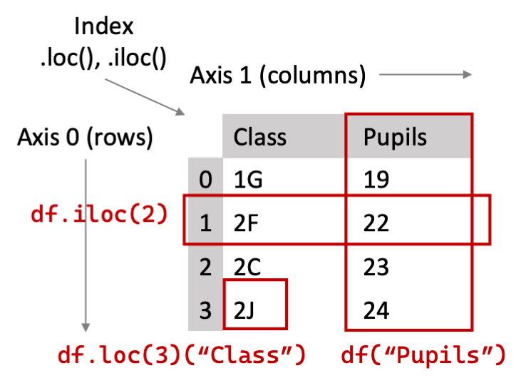
Another concept that will be introduced in the following code is finding slices of a DataFrame using pandas loc
and iloc:
locuses labels. You specify rows and columns based on their row and column labels.ilocuses integers. You specify rows and columns by their integer position values (starting from 0).
In this example we don't need the columns with URLs and large amounts of text.
The following shows examples of some ways you can remove columns:
# Remove a single column with the name 'Source for Re-opening'. The parameter axis=1 refers to a column (row would be axis=0).
df_cgd = df_cgd.drop(['Source for Re-opening'], axis=1)

# Remove the column named 'As of'
df_cgd = df_cgd.drop(['As of'], axis=1)

# Remove columns 40 and 41
df_cgd = df_cgd.drop(df_cgd.columns[[40, 41]], axis=1)

# Remove all columns between columns index 18 to 43
df_cgd = df_cgd.drop(df_cgd.iloc[:, 18:43], axis=1)

# Check the column count is now lower than the initial count
print(df_cgd.shape)
Note: you only need to keep the following columns left in the data set: Country, Code, Region, Income Group, School Closures, Date, Number of confirmed cases at time of closure, Number of cases at re-opening, Closure extended?
If you know the columns you need then rather than delete columns, you could instead selectively import the columns when
you load the data from file using the usecols= parameter:
cols = ['Country', 'Code', 'Region', 'Income Group', 'School Closures', 'Date',
        'Number of confirmed cases at time of closure', 'Number of cases at re-opening', 'Closure extended?']
df_cgd = pd.read_excel('CGD.xlsx', sheet_name='School closure tracker- Global', skiprows=1, usecols=cols)
Add related data in rows or columns
You may need to merge data. For example:
- Merging records (rows) e.g. if collected in different spreadsheets
- Merging datasets to add new variables (columns) according to the value of one or more common (index) columns
The relevant pandas methods are:
# Merge multiple data frame to add new columns
# Options for `how=` include left, right and inner.
# See https://www.w3schools.com/sql/sql_join.asp for an explanation of join types
pd.merge(df1, df2, on='name_of_common_column', how='outer')

# Concatenate multiple data frames to add rows
pd.concat([df1, df2])
In this data set we need to merge the current dataframe with data the total weeks fully closed column from the Closure/Opening Dates (Global) worksheet
col_list = ['Country', 'Total weeks FULLY CLOSED (excluding academic breaks) [red=need to verify breaks]']
df_closure = pd.read_excel('cgd.xlsx', sheet_name="Closure/Opening Dates (Global)", skiprows=1, usecols=col_list)
df_cgd_merged = pd.merge(df_cgd, df_closure, on='Country', how='outer')
Handling missing values
Missing values can be the most common feature of unclean data. These values are usually in the form of NaN or None.
There are many reasons for values to be missing, for example because they don't exist, or because of improper data collection or improper data entry.
There are different ways to deal with missing values:
- Do nothing (this may be appropriate in some circumstances).
- If your data set is large enough and/or the percentage of missing values is high, you may choose to delete the rows and columns that contain the missing data;
- Use an imputation technique to fill the missing values (e.g. mean, median, most frequent etc.)
The decision will depend on the type of data, the actions you want to perform on the data, and the reasons for the missing values.
This article on Towards Data Science gives pros and cons of some common imputation techniques. You are not expected to understand the specific imputation techniques and make an informed choice to apply to your coursework. For this course it is sufficient that you understand the implications of missing data and that you state your decision i.e. whether to do nothing, remove data or use imputation.
Identify null values
Pandas has functions that help to identify null values.
Try adding one of the following lines of code to see a count of None and NaN values in each column:
print(df_cgd.isnull().sum())
print(df_cgd.isna().sum())
Now try adding code to show which rows contain None or NaN values.
# isna() to select all rows with NaN under a single DataFrame column:
nulls = df_cgd[df_cgd['column'].isna()]

# isnull() to select all rows with NaN under a single DataFrame column:
nulls = df_cgd[df_cgd['column'].isnull()]

# isna() to select all rows with NaN in an entire DataFrame:
nulls = df_cgd[df_cgd.isna().any(axis=1)]

# isnull() to select all rows with NaN in an entire DataFrame:
df_cgd[df_cgd.isnull().any(axis=1)]
We know from the summary data that the dataset has 228 rows and that the Country column has 218 non-null values, so we assume there are 10 rows that don't have a country name. Let's look for these using one of the above methods:
nulls = df_cgd[df_cgd['Country'].isna()]
print(nulls)
It appears all the columns are null then we can remove rows 218 to 227. How to remove rows will be covered later.
A note on modifying dataframe contents
When using pandas, actions that change the data in the dataframe usually create a copy. To write the changes to the original dataframe name you need to use syntax like the following pseudocode, that is you reassign the results of the action to the same (or new) variable name:
df_new = df_original.some_operation()
In some cases using the parameter inplace=True will perform the action on the original dataframe. This will work in
some cases but not all, and the reasons are beyond this guide. Safest is probably to remember to reassign the dataframe
when you modify the contents.
Drop null values
To drop null values, dropna
will drop all the rows in which any null value is present. You can control this behavior with the 'how' parameter,
either how=any or how=all:
df.dropna()
You can also use drop with a condition rather than dropna, df.drop(df[somecondition].index, inplace=True)
replacing somecondition with the relevant criteria. For example:
df_cgd = df_cgd.drop(df_cgd[df_cgd['Country'].isna()].index)
Or you could keep the rows where one or more columns are not null, e.g.
df_not_null = df[df['column'].notna()]
To drop columns instead of rows use the axis=1 parameter. For example, delete all columns that have more than 50% of
the values missing:
# Print the columns showing the % of missing values
print(df.isnull().sum() / len(df))

# Drop columns that have more than 50% of the values missing
half_count = len(df) / 2
df = df.dropna(thresh=half_count, axis=1)

# If we look at the shape of the data now we should see the number of columns is reduced
print(df.shape)
Now, get rid of the rows where country is null, df.shape() is used only so you can see the row number before and after
the action:
print(df_cgd.shape)
df_cgd = df_cgd[df_cgd['Country'].notna()]
print(df_cgd.shape)
Replace null values
Sometimes you might need to replace them with some other value. This highly depends on your context and the dataset
you're currently working with. Sometimes a NaN can be replaced with a 0, sometimes it can be replaced with the mean of
the sample, and some other times you can take the closest value (e.g. method=ffill).
df.fillna({'Column A': 0, 'Column B': 99, 'Column C': df['Column C'].mean()})
df.fillna(method='ffill', axis=1)
df.fillna(method='ffill', axis=0)
Try replacing the blanks for the 'Closure extended?' column with 'Unknown'.
print(df_cgd['Closure extended?'])
df_cgd['Closure extended?'] = df_cgd['Closure extended?'].fillna('Unknown')
print(df_cgd['Closure extended?'])
Handling inconsistent values
When there are different unique values in the column, an inconsistency can occur. Examples include:
- Text data: Imagine a text field that contains 'Juvenile', 'juvenile' and ' juvenile ' in the same column, you could remove spaces and convert all data to lowercase. If there are a large number of inconsistent unique entries, you cannot manually check the closest match, in which case there are various packages that can be used (e.g. Fuzzy Wuzzy string matching).
- Date/time data: Inconsistent date format, such as dd / mm / yy and mm / dd / yy in the same column. Your date value may not be the correct data type, which will not allow you to perform actions efficiently and gain insight from it.
None of the CGD columns have a suitable example of inconsistent data so for this example let's first create a small data frame to work with.
name_data = [['Rio', 'M', 31, 'IT'], ['Maz', 'M', 32, 'IT'], ['Tom', 'M', 35, 'I T'], ['Nick', 'M', 34, 'IT'],
             ['Julius', 'm', 340, 'IT '], ['Julia', 'F', 31, ' IT'], ['Tom', 'male', 35, 'IT'],
             ['Nicola', 'F', 31, 'IT '],
             ['Julia', 'F', 31, 'IT'], ]
df_names = pd.DataFrame(name_data, columns=['Name', 'Gender', 'Age', 'Department'])
print(df_names)
Identify unique values
Find out what the unique values are for a field:
print(df_names['Gender'].unique())
Find out how many times a value appears:
print(df_names['Gender'].value_counts())
Replace values
If you know what you want to replace it with then use:
df_names['Gender'] = df_names['Gender'].replace('m', 'M')
or use a dictionary of values to replace multiple values:
df_names['Gender'] = df_names['Gender'].replace({'m': 'M', 'male': 'M'})
To find values outside an accepted range, for example where the age is greater than 100:
print(df_names[df_names['Age'] > 100])
If you have many columns to replace, you could apply it at "DataFrame level":
df_names.replace({
    'Gender': {
        'male': 'M',
        'm': 'M'
    },
    'Age': {340: 34}
}, inplace=True)
Find and replace duplicates
Another issue you may experience is finding and replacing duplicates. The following identified rows where all columns are duplicated
# Shows that the last row is a duplicate, though it doesn't identify the row it duplicates
print(df_names.duplicated())
Dropping duplicates try one of the following methods:
df_names = df_names.drop_duplicates()
# or
df_names = df_names.drop_duplicates(subset=['Name'])
# or
df_names = df_names.drop_duplicates(subset=['Name'], keep='last')
Remove blank spaces
Removing blank spaces (e.g. 'IT ' or 'I T') can be achieved with strip (lstrip and rstrip also exist) or just
replace:
df_names['Department'].str.strip()
df_names['Department'].str.replace(' ', '')
This isn't an exhaustive list, you may need to look through documentation and forums to identify solutions for your specific issues.
Handling classified data
Machine learning generally uses numeric values. However, datasets typically contain string or character data. Some non-numeric data can be categorised (e.g. gender), i.e. categorical values. In most cases, the categorical values are discrete and can be encoded as dummy variables, assigning a number to each category. For example rather than Yes/No as values you may replace these with 1/2 where 1=Yes and 2=No. There are tools for doing this such as the SciKit Learn One Hot Encoder.
Let's use pandas to change the values of df_cgd['Closure extended?'] from Yes, No and Unknown to 1, 2 and 3.
df_cgd['Closure extended?'] = df_cgd['Closure extended?'].replace({'Yes': 1, 'No': 2, 'Unknown': 3})
Check the data types of columns
print(df.info(verbose=True))
# or
print(df.dtypes)
The above code will show the data types of each column.
Many of the columns in this dataset will be shown as object when you want them to be numeric or date.
Pandas provides ways to convert from various data types e.g.
# Convert a field to a date time
df_cgd['Date reopening process started'] = pd.to_datetime(df_cgd['Date reopening process started'])

# Convert a field from object to numeric, the first step removes the ',' from the numbers
df_cgd['Number of cases at re-opening'] = df_cgd['Number of cases at re-opening'].str.replace(',', '')
df_cgd['Number of cases at re-opening'] = pd.to_numeric(df_cgd['Number of cases at re-opening'])
It may be easier to specify the data types when you first import the data e.g.
df = pd.read_csv('data.csv', dtype={'x1': int, 'x2': str, 'x3': int, 'x4': str})
Save the dataset
Save the prepared data set to a new .csv or .xlsx file to separate it from the original data. This ensures that you still have the raw data in case you need to return it.
# Save the DataFrame back to a new csv. 'index=False' indicates that row names should not be saved.
df_cgd.to_csv("cgd_cleaned.csv", index=False)
You can save to other formats e.g. df.to_excel, df.to_json, df.to_sql and more.
Exploring and understanding the data
Creating charts to explore the data
The code already given in basic data information and statistics will give you some understanding of the data.
To explore the data it can be also be useful to visualise it using charts. These are not your final charts. They are meant to be 'quick and dirty' i.e. don't spend time on formatting, they just need to be good enough to help you understand the data.
To create the charts
use pandas.DataFrame.plot
which in turn relies on features in matplotlib to render the charts.
This means you will need the following import in addition to pandas:
import matplotlib.pyplot as plt
Note: In PyCharm I recently experienced issues running code that previously worked using only the above import and resolved this by adding:
import matplotlib

matplotlib.use('TkAgg')
import matplotlib.pyplot as plt
To see the charts you create varies create the chart and then show it e.g.:
import pandas as pd
import numpy as np
import matplotlib.pyplot as plt

np.random.seed(1234)
df = pd.DataFrame(np.random.randn(10, 4), columns=['Col1', 'Col2', 'Col3', 'Col4'])
boxplot = df.boxplot(column=['Col1', 'Col2', 'Col3'])
boxplot.plot()
plt.show()
In PyCharm the charts are displayed in a new panel within the IDE layout.
In VS Code this displays the charts as separate pop-up windows. You can also run the code in an Interactive Window like
a jupyter notebook. To do this you need to install ipykernel pip install ipykernel. You can then run the code by
right-clicking on the file in the Explorer and selecting Run Current File in Interactive Window.
Outliers
An outlier is a data point that is significantly different from other data points in a data set
Identifying outliers
Identifying outliers is subjective and techniques include:
- Plot the data (e.g. histogram, scatter plot, boxplot)
- Use common sense
- Use statistical tests
Since this course doesn't expect any knowledge or, nor teach any, statistics then we will check for outliers by creating a chart, or plot, instead. In this instance let's create a boxplot .
This example explore the 'Cases at closure' column.
# Add this import if using PyCharm
import matplotlib.pyplot as plt

df_cgd.boxplot(column=['Cases at closure'])
plt.show()
You should now see a box plot that looks something like this:
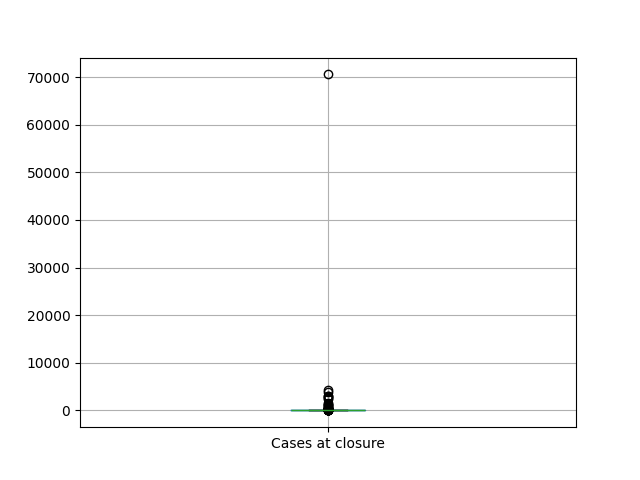
In this case there is one outlier at 70000. We can find that particular row using:
print(df_cgd.loc[df_cgd['Cases at closure'] > 70000])
The .loc function is documented here.
Dealing with outliers
It will depend on what you want to do with the data whether you wish to remove the outlier or not.
Sometimes they indicate a mistake in data collection, other time they can influence a data set, so it’s important to keep them to better understand the big picture. A rule of thumb would be:
- Drop if it’s wrong, you have a lot of data, you can go back to the data point if needed
- Don’t drop if the results are critical and a small change matters, there are a lot of outliers
Methods for handling outliers include:
- Trim the data set by deleting any points outside a set range for what is considered valid
- Replace outliers with the nearest "good" data (Winsorization)
- Replace outliers with the mean or median for that variable to avoid a missing data point
- Run two analyses: one with the outliers in and one without
- Transform the data or use forms of analysis that are more resistant to outliers e.g. Principal Component Analysis
If you run the line of code print(df_cgd.loc[df_cgd['Cases at closure'] > 70000]) then you should see that the row
relates to China. It isn't surprising given the size of the country and its population that China is an outlier. It
might however raise a question whether our chart should display cases per 1,000,000 population for example rather than
an absolute number of cases.
If you wanted to see the boxplot without China you could drop the row with index 41 (China) using:
df_cgd_ex_china = df_cgd.drop([41])
Create a histogram
A histogram shows the number of occurrences of different values in a dataset and can be useful as it reveals more than the basic stats might.
plt.hist(df['Cases at closure'])
plt.show()
Other chart types
Depending on the nature of your data set you may find other chart formats more useful such as a scatter plot. For the coursework you can consider any chart type you find useful to explore your particular data set.
Code challenges
See if you can write code to achieve one or more of the following:
- Check for outliers in other variables e.g. 'Cases at open' or 'Closure duration'
- Create a histogram for another variable e.g. 'Cases at open' or 'Closure duration'
- Create a bar chart to show the number of countries closing on each date in March 2020
- The examples in this guide use a procedural style of code. Could you write Python functions so that your some of your preparation can be applied to different data sets?
Some potential solutions:
Further information
Please refer to the reading list for tutorials and guides.